librosa.feature
2021. 4. 3. 15:02ㆍ민공지능/음성 인식 프로젝트
librosa.feature.chroma_stft
리턴 값
- chromagram : np.ndarray [shape=(n_chroma, t)]
- Normalized energy for each chroma bin at each frame.
librosa.feature.chroma_stft(y=None, sr=22050, S=None, norm=inf,
                            n_fft=2048, hop_length=512, win_length=None,
                            window='hann', center=True, pad_mode='reflect',
                            tuning=None, n_chroma=12, **kwargs)
import librosa
y1, sr1 = librosa.load('C:/nmb/nmb_data/we/testvoice_F2.wav')
y2, sr2 = librosa.load('C:/nmb/nmb_data/we/testvoice_M2.wav')
print('------------------------------------- F2 --------------------------------')
F2 = librosa.feature.chroma_stft(y=y1, sr=sr1)
print(F2,'\n')
print('------------------------------------- M2 --------------------------------')
M2 = librosa.feature.chroma_stft(y=y2, sr=sr2)
print(M2)------------------------------------- F2 --------------------------------
[[0.396835 0.9509024 0.62704265 ... 0.96180594 0.6771115 1. ]
[0.5595164 0.56608325 0.32441062 ... 1. 1. 0.61923474]
[0.82637715 0.5664801 0.19449201 ... 0.47367 0.5831766 0.5278519 ]
...
[0.32984468 0.45838016 0.3356733 ... 0.11650825 0.12122409 0.3857527 ]
[0.30277738 0.5811703 0.4861608 ... 0.20466566 0.16854385 0.37516403]
[0.3598846 1. 1. ... 0.5388965 0.37338936 0.7343799 ]]
------------------------------------- M2 --------------------------------
[[0.320811 0.8521901 0.3226452 ... 0.519334 0.2843659 0.31706065]
[0.8733224 1. 0.3479557 ... 0.50070244 0.45969787 0.7032699 ]
[1. 0.64285 0.38773406 ... 0.3362854 0.5863114 1. ]
...
[0.28075776 0.32402772 0.17749807 ... 0.5764568 0.15660381 0.15129744]
[0.32388473 0.3296805 0.16664815 ... 0.43759975 0.12112975 0.11995168]
[0.35125867 0.4362459 0.19649978 ... 0.3851469 0.17001188 0.1909172 ]]
Use an energy (magnitude) spectrum instead of power spectrogram
import numpy as np

print('------------------------------------- F2 --------------------------------')
S = np.abs(librosa.stft(y1))
chroma = librosa.feature.chroma_stft(S=S, sr=sr1)
print(chroma)

print('------------------------------------- M2 --------------------------------')
S2 = np.abs(librosa.stft(y2))
chroma = librosa.feature.chroma_stft(S=S2, sr=sr2)
print(chroma)
------------------------------------- F2 --------------------------------
[[0.6261949  0.91057926 0.72408867 ... 1.         1.         0.89434737]
 [0.65991575 0.83085966 0.69741863 ... 0.8362516  0.86821115 0.5946648 ]
 [0.7297811  0.810175   0.5653448  ... 0.6596761  0.6505265  0.55586576]
 ...
 [0.6060489  0.71759284 0.5359551  ... 0.59238815 0.61018187 0.59590757]
 [0.6535583  0.846398   0.7975717  ... 0.6383842  0.6401624  0.6294406 ]
 [0.62925166 1.         1.         ... 0.7700078  0.7793087  0.80759364]]
------------------------------------- M2 --------------------------------
[[0.5898614  0.8389981  0.6789335  ... 0.98785317 0.79714036 0.72370875]
 [1.         1.         0.70856714 ... 0.9131137  0.8308513  0.95119154]
 [0.9193935  0.7591716  0.7001591  ... 0.6737147  0.8191026  1.        ]
 ...
 [0.5756029  0.6535464  0.5628149  ... 0.9026286  0.6464118  0.62232757]
 [0.6816064  0.72203594 0.60280424 ... 0.71810246 0.6221709  0.50943226]
 [0.6361286  0.71959674 0.636623   ... 0.7606331  0.7049503  0.62486804]]
Use a pre-computed power spectrogram with a larger frame
print('------------------------------------- F2 --------------------------------')
S = np.abs(librosa.stft(y1, n_fft=4096))**2
chroma = librosa.feature.chroma_stft(S=S, sr=sr1)
print(chroma)
print('------------------------------------- M2 --------------------------------')
S2 = np.abs(librosa.stft(y2, n_fft=4096))**2
chroma = librosa.feature.chroma_stft(S=S2, sr=sr2)
print(chroma)
------------------------------------- F2 --------------------------------
[[0.52672386 0.4230828 0.5068477 ... 0.9206504 0.8201677 1. ]
[0.40589955 0.28223276 0.4675236 ... 0.9367617 0.81959593 0.78819805]
[0.42197207 0.23166715 0.25805128 ... 0.6026466 0.37012726 0.39854443]
...
[0.24756855 0.25426778 0.17463636 ... 0.20387807 0.1307967 0.13892254]
[0.6394133 0.40600616 0.32898432 ... 0.3540341 0.25533643 0.1554416 ]
[1. 1. 1. ... 0.72717553 0.3416589 0.3428477 ]]
------------------------------------- M2 --------------------------------
[[0.5679883 0.3049031 0.4796314 ... 0.07703099 0.14651535 0.2166903 ]
[1. 0.61297625 0.8983419 ... 0.17519206 0.28241155 0.55001575]
[0.6974484 0.34074524 0.47776666 ... 0.11359259 0.15029877 0.4832045 ]
...
[0.2743955 0.14617746 0.17197248 ... 1. 1. 0.36958084]
[0.19830486 0.10847064 0.09904818 ... 0.8998595 0.56046367 0.22006239]
[0.3147402 0.13615249 0.19195053 ... 0.15279983 0.104303 0.14604695]그래프 비교
import matplotlib.pyplot as plt
import librosa.display
import matplotlib as mpl
Chromagram_F2 = librosa.feature.chroma_stft(y1, sr=sr1)
mpl.rcParams["font.size"] = 20
plt.figure(figsize=(16, 6))
librosa.display.specshow(Chromagram_F2, x_axis='time', y_axis='chroma', )
plt.title('chroma_stft_F2')
plt.colorbar()
plt.show()
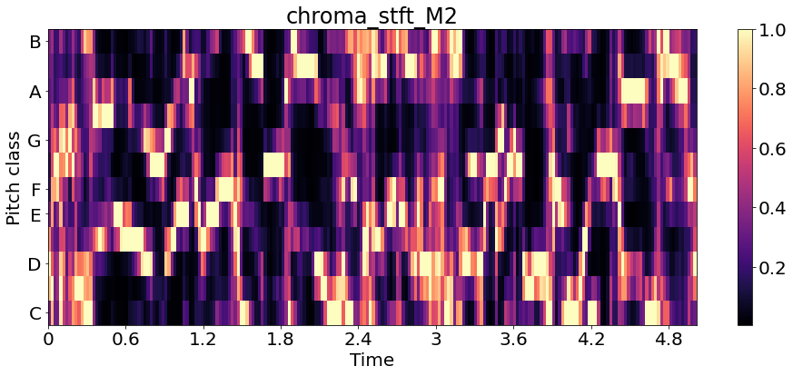
Chromagram_M2 = librosa.feature.chroma_stft(y2, sr=sr2)
mpl.rcParams["font.size"] = 20
plt.figure(figsize=(16, 6))
librosa.display.specshow(Chromagram_M2, x_axis='time', y_axis='chroma', )
plt.title('chroma_stft_M2')
plt.colorbar()
plt.show()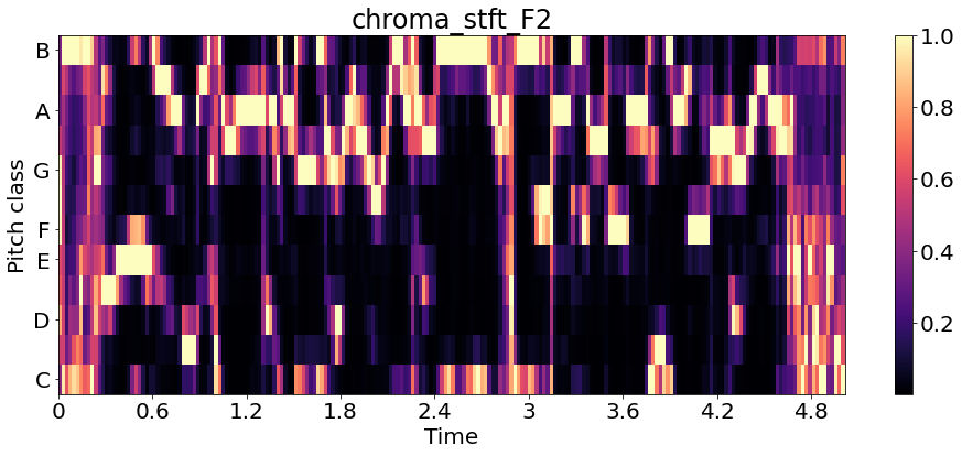
librosa.feature.chroma_cqt
리턴 값
- chromagram : np.ndarray [shape=(n_chroma, t)]
- The output chromagram
librosa.feature.chroma_cqt(y=None, sr=22050, C=None, hop_length=512,
                          fmin=None, norm=inf, threshold=0.0, tuning=None,
                          n_chroma=12, n_octaves=7, window=None,
                          bins_per_octave=36, cqt_mode='full')
chroma_cqt = librosa.feature.chroma_cqt(y=y1, sr=sr1)
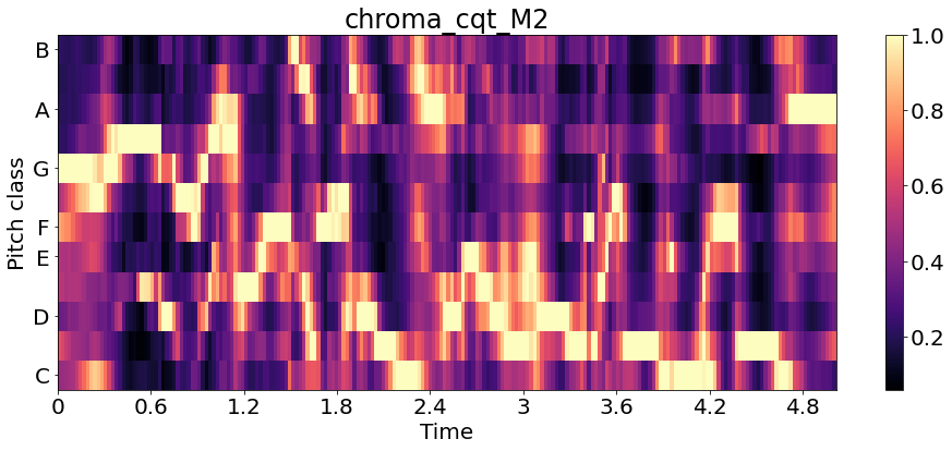
chroma_cqt2 = librosa.feature.chroma_cqt(y=y2, sr=sr2)
mpl.rcParams["font.size"] = 20
plt.figure(figsize=(16, 6))
librosa.display.specshow(chroma_cqt, x_axis='time', y_axis='chroma', )
plt.title('chroma_cqt_F2')
plt.colorbar()
plt.show()
mpl.rcParams["font.size"] = 20
plt.figure(figsize=(16, 6))
librosa.display.specshow(chroma_cqt2, x_axis='time', y_axis='chroma', )
plt.title('chroma_cqt_M2')
plt.colorbar()
plt.show()
librosa.feature.chroma_cens(Chroma Energy Normalized)
리턴값
- cens : np.ndarray [shape=(n_chroma, t)]
- The output cens-chromagram

librosa.feature.chroma_cens(y=None, sr=22050, C=None, hop_length=512,
                            fmin=None, tuning=None, n_chroma=12, n_octaves=7,
                            bins_per_octave=36, cqt_mode='full', window=None,
                            norm=2, win_len_smooth=41, smoothing_window='hann')
chroma_cens = librosa.feature.chroma_cens(y=y1, sr=sr1)
chroma_cens2 = librosa.feature.chroma_cens(y=y2, sr=sr2)
mpl.rcParams["font.size"] = 20
plt.figure(figsize=(16, 6))
librosa.display.specshow(chroma_cens, x_axis='time', y_axis='chroma', )
plt.title('chroma_cens_F2')
plt.colorbar()
plt.show()
mpl.rcParams["font.size"] = 20
plt.figure(figsize=(16, 6))
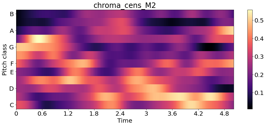
librosa.display.specshow(chroma_cens2, x_axis='time', y_axis='chroma', )
plt.title('chroma_cens_M2')
plt.colorbar()
plt.show()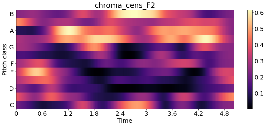
librosa.feature.melspectrogram
귀의 구조로 인한 차이
출처: https://hyongdoc.tistory.com/402 [Doony Garage]
- 사람은 500Hz와 1000Hz 소리는 쉽게 구분할 수 있지만, 10000Hz와 10500Hz는 같은 500Hz 간격임에도 불구하고 구분하기 어렵다.
- 동일한 세기로 100Hz 소리를 들려줄 때와, 10000Hz 소리를 들려줄 때 사람이 느끼는 세기는 다르다.
mel-scale은 이러한 사람의 귀를 칼라 맵인 스펙트로그램에 반영하는 것을 의미한다.
(고주파로 갈수록 같은 mel 값을 가지는 주파수 범위가 넓어진다.)
리턴 값 :
- S : np.ndarray [shape=(n_mels, t)]
- Mel spectrogram
librosa.feature.melspectrogram(y=None, sr=22050, S=None, n_fft=2048,
                              hop_length=512, win_length=None, window='hann',
                              center=True, pad_mode='reflect', power=2.0, **kwargs)
print('------------------------------------- F2 --------------------------------')
F2 = librosa.feature.melspectrogram(y=y1, sr=sr1)
print(F2,'\n')
print('------------------------------------- M2 --------------------------------')
M2 = librosa.feature.melspectrogram(y=y2, sr=sr2)
print(M2)------------------------------------- F2 --------------------------------
[[1.28955115e-02 1.11121126e-02 7.33756321e-03 ... 2.49373000e-02
5.45657203e-02 3.73395756e-02]
[2.18119714e-02 7.78498650e-02 1.61865473e-01 ... 4.00794268e-01
4.16311264e-01 1.90331221e-01]
[1.51729211e-02 3.15802321e-02 5.53060099e-02 ... 1.84591115e-01
1.30545422e-01 1.57961607e-01]
...
[3.61378056e-08 4.28206519e-08 3.49686573e-08 ... 1.05480865e-06
1.03485945e-06 1.73392277e-06]
[5.06456477e-09 9.70210134e-09 9.30362987e-09 ... 1.14749675e-07
1.76064859e-07 6.96718416e-07]
[4.13563989e-10 6.33965547e-10 6.10381024e-10 ... 1.92417762e-08
3.16240651e-08 2.52590354e-07]]
------------------------------------- M2 --------------------------------
[[2.3119669e-02 3.1757120e-02 2.8043669e-02 ... 4.6432182e-01
4.3421051e-01 2.9909253e-01]
[2.0760961e-02 6.1749190e-02 8.5803375e-02 ... 9.2933339e-01
1.0508763e+00 1.0738103e+00]
[3.8493581e-03 7.7256500e-03 1.2649094e-02 ... 6.2744021e-01
3.4037867e-01 9.0059072e-01]
...
[1.2186531e-07 1.9294495e-07 1.8853085e-07 ... 4.8735046e-06
1.7241197e-06 1.4671884e-06]
[8.9550710e-08 8.5921762e-08 6.7769577e-08 ... 3.7791659e-07
3.9809882e-07 8.7064046e-07]
[4.9952547e-08 1.5936049e-08 4.1547974e-09 ... 1.7301943e-08
2.8796848e-08 1.4198044e-07]]D = np.abs(librosa.stft(y1))**2
S = librosa.feature.melspectrogram(S=D, sr=sr1)
S = librosa.feature.melspectrogram(y=y1, sr=sr1, n_mels= 512,fmax=sr1/2)
import matplotlib.pyplot as plt
fig, ax = plt.subplots()
S_dB = librosa.power_to_db(S, ref=np.max)
img = librosa.display.specshow(S_dB, x_axis='time',
y_axis='mel', sr=sr1,
fmax=sr1/2, ax=ax)
fig.colorbar(img, ax=ax, format='%+2.0f dB')
ax.set(title='melspectrogram_F2')
D = np.abs(librosa.stft(y2))**2
S = librosa.feature.melspectrogram(S=D, sr=sr2)
S = librosa.feature.melspectrogram(y=y2, sr=sr2, n_mels=512,fmax=sr2/2)
import matplotlib.pyplot as plt
fig, ax = plt.subplots()
S_dB = librosa.power_to_db(S, ref=np.max)
img = librosa.display.specshow(S_dB, x_axis='time',
y_axis='mel', sr=sr2,
fmax=sr2/2, ax=ax)
fig.colorbar(img, ax=ax, format='%+2.0f dB')
ax.set(title='melspectrogram_M2')* n_mels = 칼라 맵의 주파수 해상도
(mel 기준으로 몇 개의 값으로 표현할지 나타내는 변수, 많으면 많을수록 필터를 촘촘하게 쓰는 것과 같아서 stft로 표현한 칼라 맵과 유사한 형태가 된다)


'민공지능 > 음성 인식 프로젝트' 카테고리의 다른 글
| STT (0) | 2021.04.26 |
|---|---|
| Speech VGG (0) | 2021.04.25 |
| 음성 데이터2(Mel Spectrogram, MFCCs, Chroma Frequencies) (0) | 2021.04.03 |
| 음성 데이터 (오디오 파일 이해, 2D Sound Waves, Fourier Transform, Spectrogram) (0) | 2021.04.03 |