2021. 5. 1. 23:53ㆍ민공지능/캐글 & 데이콘
캐글에서 열린 [Tabular Playground Series - Apr 2021]대회에 참가했다.
www.kaggle.com/c/tabular-playground-series-apr-2021
'The dataset is used for this competition is synthetic but based on a real dataset (in this case, the actual Titanic data!) and generated using a CTGAN. The statistical properties of this dataset are very similar to the original Titanic dataset, but there's no way to "cheat" by using public labels for predictions. How well does your model perform on truly private test labels?'
Goal : Your task is to predict whether or not a passenger survived the sinking of the Synthanic (a synthetic, much larger dataset based on the actual Titanic dataset). For each PasengerId row in the test set, you must predict a 0 or 1 value for the Survived target. Your score is the percentage of passengers you correctly predict. This is known as accuracy.
타이타닉 침몰에서 승객이 살아남았는지 예측하는 대회다.
테스트셋의 각 승객 ID 행의 생존 목표값에 대해 0또는 1값을 예측해야 한다.


survival : 생존여부 ( 0 = 죽음, 1 = 생존)
pclass : 티켓 클래스(1=1위, 2=2위, 3=3위)
sex : 성별
age : 나이 (1살 미만이면 분수로 표현, xx.5의 형태)
sibsp : 타이타닉호에 탑승한 형제자매 수 / 배우자 수
parch : 타이타닉호에 탑승한 부모 / 아이들의 수
ticket : 티켓번호
fare : 운임승차료
cabin : 객실 번호
embarked : 출항지(C = Cherbourg, Q = Queenstown, S = Southampton)

<train>
       PassengerId  Survived  Pclass                Name     Sex    Age  SibSp  Parch     Ticket   Fare   Cabin Embarked
0                0         1       1    Oconnor, Frankie    male    NaN      2      0     209245  27.14  C12239        S
1                1         0       3         Bryan, Drew    male    NaN      0      0      27323  13.35     NaN        S
2                2         0       3      Owens, Kenneth    male   0.33      1      2  CA 457703  71.29     NaN        S
3                3         0       3       Kramer, James    male  19.00      0      0   A. 10866  13.04     NaN        S
4                4         1       3       Bond, Michael    male  25.00      0      0     427635   7.76     NaN        S
...            ...       ...     ...                 ...     ...    ...    ...    ...        ...    ...     ...      ...
99995        99995         1       2         Bell, Adele  female  62.00      0      0   PC 15008  14.86  D17243        C
99996        99996         0       2       Brown, Herman    male  66.00      0      0      13273  11.15     NaN        S
99997        99997         0       3  Childress, Charles    male  37.00      0      0        NaN   9.95     NaN        S
99998        99998         0       3    Caughlin, Thomas    male  51.00      0      1     458654  30.92     NaN        S
99999        99999         0       3       Enciso, Tyler    male  55.00      0      0     458074  13.96     NaN        S
<test>
       PassengerId  Pclass                Name     Sex   Age  SibSp  Parch    Ticket    Fare   Cabin Embarked  Survived
0           100000       3    Holliday, Daniel    male  19.0      0      0     24745   63.01     NaN        S         0
1           100001       3    Nguyen, Lorraine  female  53.0      0      0     13264    5.81     NaN        S         1
2           100002       1     Harris, Heather  female  19.0      0      0     25990   38.91  B15315        C         1
3           100003       2        Larsen, Eric    male  25.0      0      0    314011   12.93     NaN        S         0
4           100004       1       Cleary, Sarah  female  17.0      0      2     26203   26.89  B22515        C         1
...            ...     ...                 ...     ...   ...    ...    ...       ...     ...     ...      ...       ...
99995       199995       3       Cash, Cheryle  female  27.0      0      0      7686   10.12     NaN        Q         1
99996       199996       1       Brown, Howard    male  59.0      1      0     13004   68.31     NaN        S         0
99997       199997       3  Lightfoot, Cameron    male  47.0      0      0   4383317   10.87     NaN        S         0
99998       199998       1  Jacobsen, Margaret  female  49.0      1      2  PC 26988   29.68  B20828        C         1
99999       199999       1    Fishback, Joanna  female  41.0      0      2  PC 41824  195.41  E13345        C         1
all_df = pd.concat([train, test]).reset_index(drop=True)
# train과 test의 dataframe을 합쳐준 뒤, 기존 인덱스를 버리고 재배열 해준다.
target = train.pop('Survived')
# train의 'Survived' 열 부분을 pop()으로 삭제해주고, 꺼낸 'Survived'요소는 target으로 설정한다.
# 결측값 확인
print(all_df.isnull().sum())
'''
PassengerId 0
Survived 0
Pclass 0
Name 0
Sex 0
Age 6779
SibSp 0
Parch 0
Ticket 9804
Fare 267
Cabin 138697
Embarked 527
'''
all_df['Age'] = all_df['Age'].fillna(all_df['Age'].mean())
# fillna()함수는 결측값을 대체해주는 함수다. mean을 쓰면 평균값으로 대체해준다.
all_df['Cabin'] = all_df['Cabin'].fillna('X').map(lambda x: x[0].strip())
# 객실 열들의 결측값에는 'X' 로 채우고 값이 있으면 0번째인 알파벳만 불러온다.
# .strip()을 해주면 양쪽 끝에 있는 공백과 \n 기호를 삭제시켜 준다.
all_df['Ticket'] = all_df['Ticket'].fillna('X').map(lambda x:str(x).split()[0] if len(str(x).split()) > 1 else 'X')
# 티켓 열의 결측값에 'X'로 채우고 값이 있는 경우, 공백 기준으로 문자를 나누었을 때
# 나눈 str형태의 문자의 길이가 1보다 크면 str의 (공백 기준으로) 0번째만 지정하고 아니면 'X'로 바꾼다.
fare_map = all_df[['Fare', 'Pclass']].dropna().groupby('Pclass').median().to_dict()
# 운임승차료와 티겟 클래스의 데이터프레임을 리스트로 만들어주고 dropna()를 통해 결측치를 삭제한다.
# groupby('Pclass')는 'Pclass'를 제외한 컬럼에 함수 적용하게 해준다.
# Fare(운임승차료)의 중앙값을 Pclass에 맞춰서 뽑아내고, dictionary형태로 만들어준다.
# 실행 결과 : {'Fare': {1: 71.81, 2: 21.7, 3: 11.33}}
all_df['Fare'] = all_df['Fare'].fillna(all_df['Pclass'].map(fare_map['Fare']))
# 'Fare'의 결측값을 위의 fare_map에서 처리한 Fare의 값으로 채워준다.
all_df['Fare'] = np.log1p(all_df['Fare'])
# 정규화를 해주기 위해 np.log1p를 해준다.
# np.log가 아닌 log1p를 하는 이유는 price가 0이 되는 경우 y 값이 무한대가 되버리기 때문에 정규화가 힘들어진다.
# 그래서 log1p를 사용하는 것이다. = log(1+ax)
all_df['Embarked'] = all_df['Embarked'].fillna('X')
# 출항지의 결측값도 'X'로 채워준다.
all_df['Name'] = all_df['Name'].map(lambda x: x.split(',')[0])
# 이름의 경우 ','를 기준으로 나눠 0번째만 가져온다.(surnames = 성씨)
Feature engeenring 후
print(all_df[:10])
'''
   PassengerId  Survived  Pclass     Name     Sex        Age  SibSp  Parch Ticket      Fare Cabin Embarked
0            0         1       1  Oconnor    male  34.464565      2      0      X  3.337192     C        S
1            1         0       3    Bryan    male  34.464565      0      0      X  2.663750     X        S
2            2         0       3    Owens    male   0.330000      1      2     CA  4.280686     X        S
3            3         0       3   Kramer    male  19.000000      0      0     A.  2.641910     X        S
4            4         1       3     Bond    male  25.000000      0      0      X  2.170196     X        S
5            5         0       2  Sassano    male  35.000000      0      0      X  2.042518     X        S
6            6         0       3   Conway    male   7.000000      0      0      X  2.376764     X        S
7            7         1       3   Werner  female   6.000000      1      2      X  3.481240     X        S
8            8         0       1  Wardlaw    male  27.000000      2      1      X  4.304335     A        S
9            9         0       2   Greigo    male  66.000000      0      0      X  2.316488     D        C
'''

print(all_df.isnull().sum())
'''
PassengerId    0
Survived       0
Pclass         0
Name           0
Sex            0
Age            0
SibSp          0
Parch          0
Ticket         0
Fare           0
Cabin          0
Embarked       0
dtype: int64
'''
# 컬럼별로 다르게 적용
label_cols = ['Name', 'Ticket', 'Sex']
onehot_cols = ['Cabin', 'Embarked']
numerical_cols = ['Pclass', 'Age', 'SibSp', 'Parch', 'Fare']
def label_encoder(c):
le = LabelEncoder() # categorical 컬럼을 숫자데이터로 변경
return le.fit_transform(c)
scaler = StandardScaler()
# 평균 0 , 분산 1로 조정한다
onehot_encoded_df = pd.get_dummies(all_df[onehot_cols])
# get_dummies = 결측값을 제외하고 0과 1로 구성된 더미들이 만들어진다.
'''
Cabin_A Cabin_B Cabin_C Cabin_D Cabin_E ... Cabin_X Embarked_C Embarked_Q Embarked_S Embarked_X
0 0 0 1 0 0 ... 0 0 0 1 0
1 0 0 0 0 0 ... 1 0 0 1 0
2 0 0 0 0 0 ... 1 0 0 1 0
3 0 0 0 0 0 ... 1 0 0 1 0
4 0 0 0 0 0 ... 1 0 0 1 0
... ... ... ... ... ... ... ... ... ... ... ...
199995 0 0 0 0 0 ... 1 0 1 0 0
199996 0 0 0 0 0 ... 1 0 0 1 0
199997 0 0 0 0 0 ... 1 0 0 1 0
199998 0 1 0 0 0 ... 0 1 0 0 0
199999 0 0 0 0 1 ... 0 1 0 0 0
[200000 rows x 13 columns]
'''
label_encoded_df = all_df[label_cols].apply(label_encoder)
# [label_cols]에 위에서 정의해준 label_encoder함수를 적용해준다.(숫자 데이터로 변경)
'''
Name Ticket Sex
0 17441 49 1
1 3063 49 1
2 17798 14 1
3 12742 0 1
4 2335 49 1
... ... ... ...
199995 3844 49 0
199996 2992 49 1
199997 13842 49 1
199998 11475 21 0
199999 7730 21 0
[200000 rows x 3 columns]
'''
numerical_df = pd.DataFrame(scaler.fit_transform(all_df[numerical_cols]), columns=numerical_cols)
# standardScaler() 적용해주면서 평균 0, 분산 1로 값들을 전처리 해준다.
'''
Pclass Age SibSp Parch Fare
0 -1.425730 -4.307127e-16 1.901268 -0.505478 0.134351
1 0.877699 -4.307127e-16 -0.539572 -0.505478 -0.533837
2 0.877699 -2.069149e+00 0.680848 1.628715 1.070483
3 0.877699 -9.374220e-01 -0.539572 -0.505478 -0.555506
4 0.877699 -5.737175e-01 -0.539572 -0.505478 -1.023540
... ... ... ... ... ...
199995 0.877699 -4.524827e-01 -0.539572 -0.505478 -0.786852
199996 -1.425730 1.487275e+00 0.680848 -0.505478 1.028715
199997 0.877699 7.598657e-01 -0.539572 -0.505478 -0.722092
199998 -1.425730 8.811005e-01 0.680848 1.628715 0.220096
199999 -1.425730 3.961612e-01 -0.539572 1.628715 2.062203
[200000 rows x 5 columns]
'''
target_df = all_df[TARGET]
# 열 단위로 집계(axis = 0), 행 단위로 집계(axis = 1)
all_df = pd.concat([numerical_df, label_encoded_df, onehot_encoded_df, target_df], axis=1)
#[200000 rows x 22 columns]

all_df_scaled = all_df.drop([TARGET], axis = 1).copy()
# all_df에서 [TARGET]의 열 부분을 삭제한 데이터 프레임을 복사한다.

scaler.fit(all_df.drop([TARGET], axis = 1))
# [TARGET]의 열 부분을 삭제한 데이터 프레임을 standardScaler로 fit 해준다.

all_df_scaled = scaler.transform(all_df_scaled)
# 복사된 데이터 프레임에 scaler.transform 해준다.
print(all_df_scaled)
'''
[[-1.42573042e+00  1.08162950e-16  1.90126811e+00 ... -2.74320022e-01
   6.47016908e-01 -5.14000153e-02]
 [ 8.77698588e-01  1.08162950e-16 -5.39572147e-01 ... -2.74320022e-01
   6.47016908e-01 -5.14000153e-02]
 [ 8.77698588e-01 -2.06914920e+00  6.80847982e-01 ... -2.74320022e-01
   6.47016908e-01 -5.14000153e-02]
 ...
 [ 8.77698588e-01  7.59865706e-01 -5.39572147e-01 ... -2.74320022e-01
   6.47016908e-01 -5.14000153e-02]
 [-1.42573042e+00  8.81100542e-01  6.80847982e-01 ... -2.74320022e-01
  -1.54555466e+00 -5.14000153e-02]
 [-1.42573042e+00  3.96161197e-01 -5.39572147e-01 ... -2.74320022e-01
  -1.54555466e+00 -5.14000153e-02]]

'''

all_df_scaled = pd.DataFrame(all_df_scaled, columns=all_df.drop([TARGET], axis = 1).columns)

X = all_df_scaled
y = all_df[TARGET]
print (f'X:{X.shape} y: {y.shape}')
# X:(200000, 21) y: (200000,)


X_train, X_test, y_train, y_test = train_test_split(
    X, y, test_size = 0.20, random_state = RANDOM_SEED)
# RANDOM_SEED = 2021

test = all_df_scaled[len(train):]
print (f'X_train:{X_train.shape} y_train: {y_train.shape}')
# X_train:(160000, 21) y_train: (160000,)
print (f'X_test:{X_test.shape} y_test: {y_test.shape}')
# X_test:(40000, 21) y_test: (40000,)
print (f'test:{test.shape}')
# test:(100000, 21)
<Single SVM>
서포트 벡터 머신(SVM)은 결정 경계(Decision Boundary), 즉 분류를 위한 기준 선을 정의하는 모델이다.
scikit-learn의 SVM을 사용하기 위해선 먼저 SVC(Support Vector Classifier) 오브젝트를 생성해야 한다.
svc_kernel_rbf = SVC(
       kernel='rbf',
       random_state=0,
       C=1.3040348958661234,
       gamma=0.11195797734572176,
       verbose=True)

svc_kernel_rbf.fit(X_train, y_train)
y_pred = svc_kernel_rbf.predict(X_test)
accuracy_score(y_pred, y_test)

final_pred = svc_kernel_rbf.predict(test)

submission['Survived'] = np.round(final_pred).astype(int)
submission.to_csv('A:\\study\\data\\titanic\\svc_kernel_rbf.csv')
svc의 kernel 종류는 linear, poly(다항), rbf(가우시안), sigmoid(시그모이드)가 있다
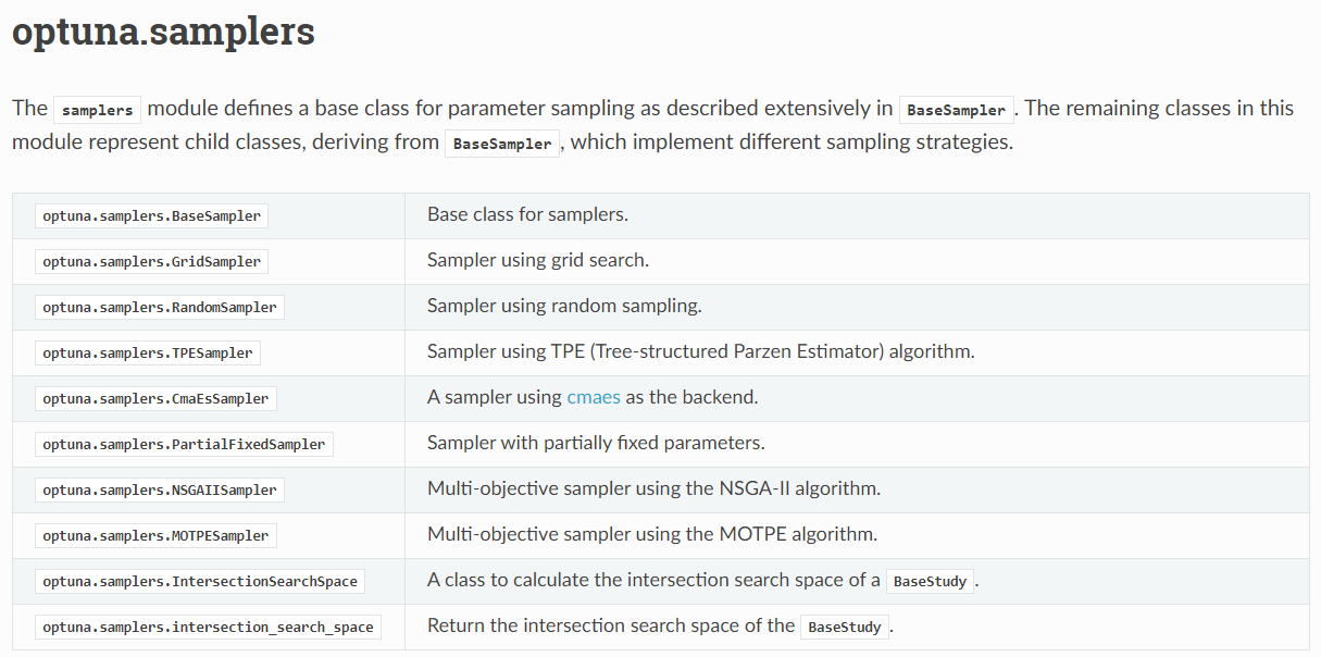
최적의 파라미터 값을 찾아주는 알고리즘인 optuna.
설치는 cmd에 pip install optuna 해주면 된다.
여러 모델을 병렬화하여 하이퍼 파라미터 최적화 분석을 해준다.
# Hyperparams selection and Kfolds==================
def objective(trial):
    from sklearn.svm import SVC
    params = {
        'C': trial.suggest_loguniform('C', 0.01, 0.1),
        'gamma': trial.suggest_categorical('gamma', ["auto"]),
        'kernel': trial.suggest_categorical("kernel", ["rbf"])
    }

    svc = SVC(**params, verbose=True)
    svc.fit(X_train, y_train)
    return svc.score(X_test, y_test)

study = optuna.create_study(sampler=optuna.samplers.TPESampler(seed=123),# TPESampler알고리즘을 사용한다.
                            direction="maximize", # 최적화 방향 = 최대화
                            pruner=optuna.pruners.MedianPruner()
                            # trial의 최상의 중간 결과가 이전 시행의 중간 결과 중위수보다 더 나쁜 경우 같은 단계에서 제거
study.optimize(objective, n_trials=5, show_progress_bar=True)
# n_trials = 시험 시도 횟수

print(f"Best Value from optune: {study.best_trial.value}")
print(f"Best Params from optune: {study.best_params}")
"""
.............
Warning: using -h 0 may be faster
*....................................................................................................................................................................................................................................................................................................................................................................................................................................
Warning: using -h 0 may be faster
*.......................
Warning: using -h 0 may be faster
*
optimization finished, #iter = 569119
obj = -48820.162701, rho = 0.083938
nSV = 47154, nBSV = 33879
Total nSV = 47154
[I 2021-05-02 15:40:54,949] A new study created in memory with name: no-name-4fe5ef73-10f1-4722-a5b3-cef2ca5d5d0e
C:\Users\sswwd\\anaconda3\envs\kaggle\lib\site-packages\optuna\progress_bar.py:47: ExperimentalWarning: Progress bar is experimental (supported from v1.2.0). The interface can change in the future.
  self._init_valid()
  0%|                                                                                             | 0/5 [00:00<?, ?it/s[
LibSVM]...................................
Warning: using -h 0 may be faster
*....
Warning: using -h 0 may be faster
*.
Warning: using -h 0 may be faster
*
optimization finished, #iter = 39786
obj = -2191.690629, rho = 0.188789
nSV = 47161, nBSV = 46401
Total nSV = 47161
[I 2021-05-02 15:54:04,721] Trial 0 finished with value: 0.87555 and parameters: {'C': 0.049712909978071915, 'gamma': 'auto', 'kernel': 'rbf'}. Best is trial 0 with value: 0.87555.
 20%|████████████████▊                                                                   | 1/5 [13:09<52:39, 789.77s/it][LibSVM]...................................
Warning: using -h 0 may be faster
*..
Warning: using -h 0 may be faster
*
optimization finished, #iter = 37389
obj = -912.380057, rho = 0.123106
nSV = 51395, nBSV = 51042
Total nSV = 51395
[I 2021-05-02 16:04:42,876] Trial 1 finished with value: 0.8744 and parameters: {'C': 0.019325882509735583, 'gamma': 'auto', 'kernel': 'rbf'}. Best is trial 0 with value: 0.87555.
 40%|█████████████████████████████████▌                                                  | 2/5 [23:47<35:01, 700.58s/it[
LibSVM]....................................
Warning: using -h 0 may be faster
*.
Warning: using -h 0 may be faster
*.
Warning: using -h 0 may be faster
*
optimization finished, #iter = 37600
obj = -805.411248, rho = 0.115731
nSV = 52153, nBSV = 51826
Total nSV = 52153
[I 2021-05-02 16:16:25,591] Trial 2 finished with value: 0.874225 and parameters: {'C': 0.016859762540733375, 'gamma': 'auto', 'kernel': 'rbf'}. Best is trial 0 with value: 0.87555.
 60%|██████████████████████████████████████████████████▍                                 | 3/5 [35:30<23:23, 701.56s/it][LibSVM]...................................
Warning: using -h 0 may be faster
*..
Warning: using -h 0 may be faster
*.
Warning: using -h 0 may be faster
*
optimization finished, #iter = 37497
obj = -1603.400322, rho = 0.168959
nSV = 48447, nBSV = 47874
Total nSV = 48447
[I 2021-05-02 16:27:28,245] Trial 3 finished with value: 0.8752 and parameters: {'C': 0.03558891673908702, 'gamma': 'auto', 'kernel': 'rbf'}. Best is trial 0 with value: 0.87555.
 80%|███████████████████████████████████████████████████████████████████▏                | 4/5 [46:33<11:26, 686.20s/it[
LibSVM]....................................
Warning: using -h 0 may be faster
*...
Warning: using -h 0 may be faster
*.
Warning: using -h 0 may be faster
*
optimization finished, #iter = 39963
obj = -2303.514547, rho = 0.190273
nSV = 46971, nBSV = 46179
Total nSV = 46971
[I 2021-05-02 16:38:23,815] Trial 4 finished with value: 0.875575 and parameters: {'C': 0.052416614815162584, 'gamma': 'auto', 'kernel': 'rbf'}. Best is trial 4 with value: 0.875575.
100%|████████████████████████████████████████████████████████████████████████████████████| 5/5 [57:28<00:00, 689.77s/it]
Best Value from optune: 0.875575
Best Params from optune: {'C': 0.052416614815162584, 'gamma': 'auto', 'kernel': 'rbf'}

"""